Introduction

Deep learning tasks can be complex and hard to measure: how do we know whether one network is better than another? In some simpler cases such as regression, the loss function used to train a network can be a good measurement of the network’s performance. However, for many real-world tasks, there are evaluation metrics that encapsulate, in a single number, how well a network is doing in terms of real world performance. These evaluation metrics allow us to quickly see the quality of a model, and easily compare different models on the same tasks.

Next, we’ll go through some case studies of different tasks and their metrics.

Warmup: Classification and the F1 Score

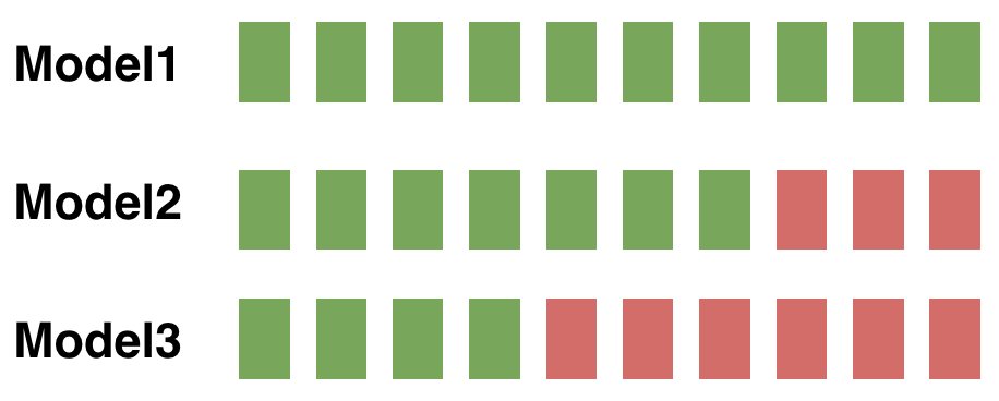
Let’s consider a simple binary classification problem, where we are trying to predict if a patient is healthy or has pneumonia. We have a test set with 10 patients, where 9 patients are healthy (shown as green squares) and 1 patient has pneumonia (shown as a red square).

Ground truth for your test set. (source)

We trained 3 models for this task (Model1, Model2, Model3), and we’d like to compare the performance of these models. The predictions from each model on the test set are shown below:

Results of your three models on the test set. (source)

Accuracy

To compare the models, we could first use accuracy, which is the number of correctly classified examples divided by the total:

\[\text{accuracy}(f) = \frac{\sum_{x_i \in X_{test}} \mathbb{1}\{f(x_i) = y_i\}}{\mid X_{test} \mid}\]

If we use accuracy as your evaluation metric, it seems that the best model is Model1.

\[\text{Accuracy}(M_1) = \frac{9}{10} \qquad \text{Accuracy}(M_2) = \frac{8}{10} \qquad \text{Accuracy}(M_3) = \frac{5}{10}\]

In general, when you have class imbalance (which is most of the time!), accuracy is not a good metric to use.

Confusion Matrix

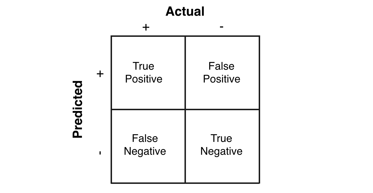
Accuracy doesn’t discriminate between errors (i.e., it treats misclassifying a patient with pneumonia as healthy the same as misclassifying a visualizing patient with having pneumonia). A confusion matrix is a tabular format for showing a more detailed breakdown of a model’s correct and incorrect classifications.

A confusion matrix for binary classification. (source)

Precision, Recall, and the F1 Score

For pneumonia detection, it is crucial that we find all the patients that have pneumonia. Predicting patients with pneumonia as healthy is not acceptable (since the patients will be left untreated). Thus, a natural question to ask when evaluating our models is:

Out of all the patients with pneumonia, how many did the model predict as having pneumonia?

This metric is recall, which is expressed as the following:

\[\text{Recall} = \frac{tp}{tp + fn}\]

What is the recall for each model?

\[\text{Recall}(M_1) = \frac{0}{1} \qquad \text{Recall}(M_2) = \frac{1}{1} \qquad \text{Recall}(M_3) = \frac{1}{1}\]

Imagine that the treatment for pneumonia is very costly and therefore you would also like to make sure only patients with pneumonia receive treatment. A natural question to ask would be:

Out of all the patients that are predicted to have pneumonia, how many actually have pneumonia?

This metric is precision, expressed as the following:

\[\text{Precision} = \frac{tp}{tp + fp}\]

What is the precision for each model?

\[\text{precision}(M_1) = \frac{0}{0} \qquad \text{precision}(M_2) = \frac{1}{3} \qquad \text{precision}(M_3) = \frac{1}{6}\]

Precision and recall are both useful, but having multiple evaluation metrics makes it difficult to directly compare models. From Andrew Ng’s machine learning book:

“Having multiple-number evaluation metrics makes it harder to compare algorithms. Better to combine them to a single evaluation metric. Having a single-number evaluation metric speeds up your ability to make a decision when you are selecting among a large number of classifiers. It gives a clear preference ranking among all of them, and therefore a clear direction for progress.” - Machine Learning Yearning

F1 score is a metric that combines recall and precision by taking their harmonic mean:

\[F_1 = 2 \cdot \frac{\text{precision} \cdot \text{recall}}{\text{precision} + \text{recall}}\]

What is the F1 score for each model?

\[F_1(M_1) = 0 \qquad F_1(M_2) = \frac{1}{2} \qquad F_1 = \frac{2}{7}\]

Food for thought: If F1 score is a great one-number measurement of model performance, why don’t we use it as the loss function?

Object Detection: IoU, AP, and mAP

In object detection, two primary metrics are used: intersection over union (IoU) and mean average precision (mAP). Let’s walk through a small example (figure credit to J. Hui’s excellent post).

Intersection over Union (IoU)

Object detection involves finding objects, classifying them, and localizing them by drawing bounding boxes around them. Intersection over union is an intuitive metric that measures the goodness of fit of a bounding box:

Intersection over Union. (source)

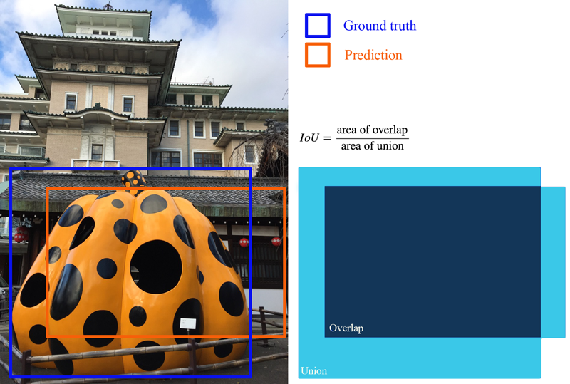The higher the IoU, the better the fit. IoU is a great metric since it works well for any size and shape of object. This per-object metric, along with precision and recall, form the basis for the full object detection metric, mean average precision (mAP).

Average Precision (AP): the Area Under Curve (AUC)

Object detectors create multiple predictions: each image can have multiple predicted objects, and there are many images to run inference on. Each predicted object has a confidence assigned with it: this is how confident the detector is in its prediction.

We can choose different confidence thresholds to use, to decide which predictions to accept from the detector. For instance, if we set the threshold to 0.7, then any predictions with confidence greater than 0.7 are accepted, and the low confidence predictions are discarded. Since there are so many different thresholds to choose, how do we summarize the performance of the detector?

The answer uses a precision-recall curve. At each confidence threshold, we can measure the precision and recall of the detector, giving us one data point. If we connect these points together, one for each threshold, we get a precision recall curve like the following:

Precision recall curve. The line is the curve: the blue shows the area under the curve (AUC). (source)

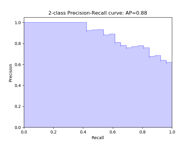The better the model, the higher the precision and recall at its points: this pushes the boundary of the curve (the dark line) towards the top and right. We can summarize the performance of the model with one metric, by taking the area under the curve (shown in blue). This gives us a number between 0 and 1, where higher is better. This metric is commonly known as average precision (AP).

Mean Average Precision (mAP)

Object detection is a complex task: we want to accurately detect all the objects in an image, draw accurate bounding boxes around each one, and accurately predict each object’s class. We can actually encapsulate all of this into one metric: mean average precision (mAP).

To start, let’s compute AP for a single image and class. Imagine our network predicts 10 objects of some class in an image: each prediction is a single bounding box, predicted class, and predicted confidence (how confident the network is in its prediction).

We start with IoU to decide if each prediction is correct or not. For a ground truth object and nearby prediction, if

1. the predicted class matches the actual class, and
2. the IoU is greater than a threshold,

we say that the network got that prediction right (true positive). Otherwise, the prediction is a false positive.

We can now sort our predictions by their confidence, descending, resulting in the following table:

Table of predictions, from most confident to least confident. Cumulative recision and recall shown on the right. (source)

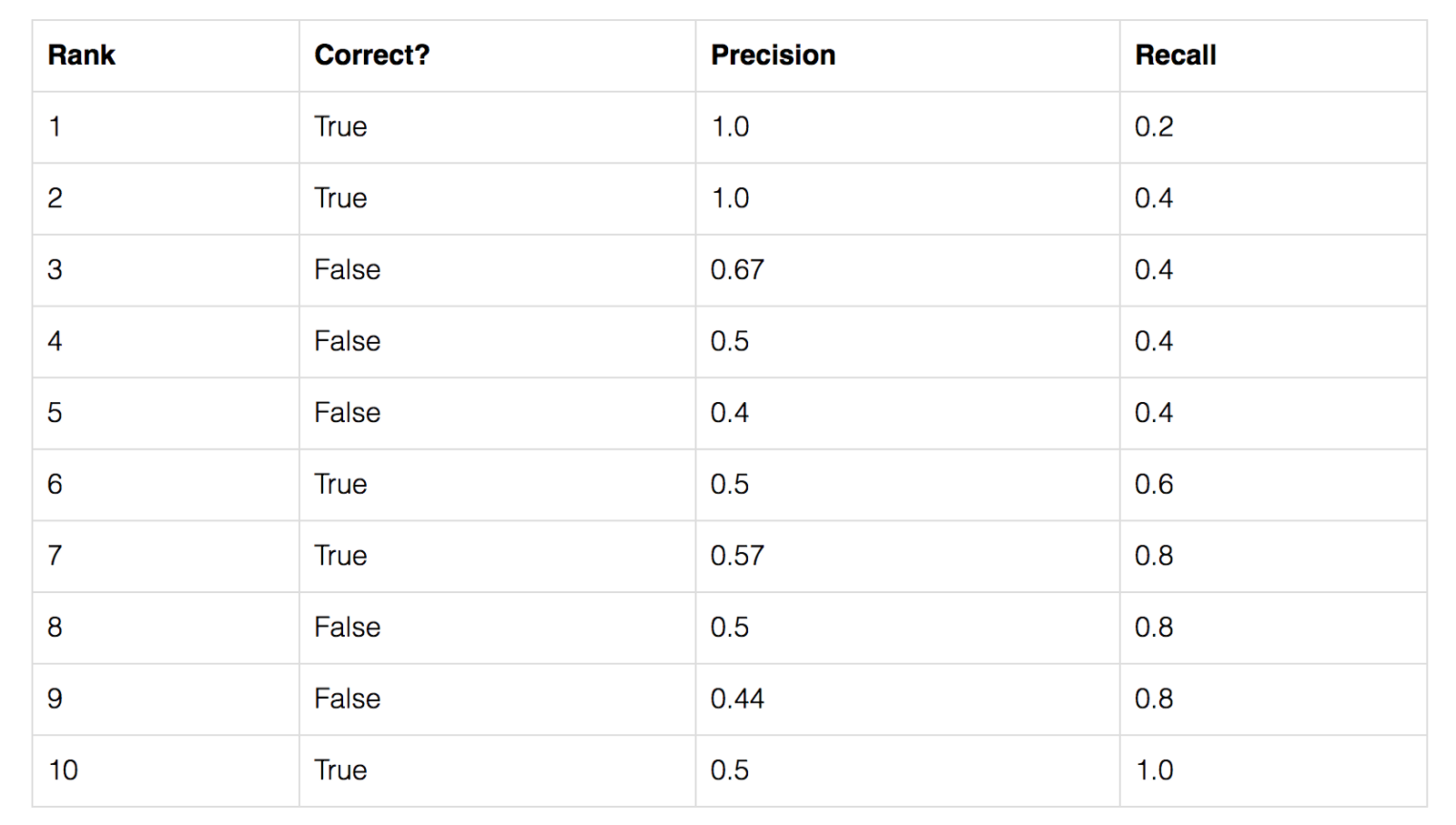For each confidence level (starting from largest to smallest), we compute the precision and recall up to that point. If we graph this, we get the raw precision-recall curve for this image and class:

The raw precision-recall curve. (source)

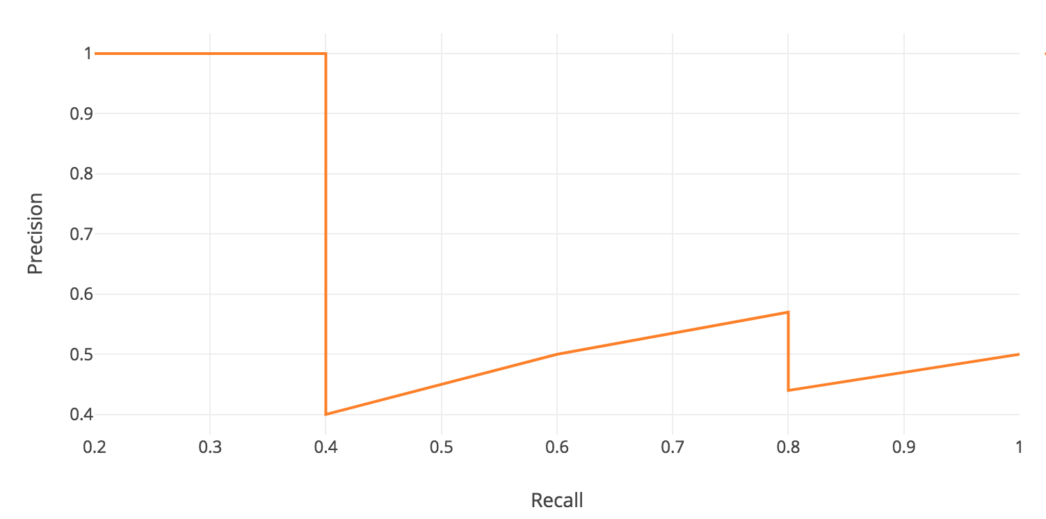Notice how our precision-recall curve is jagged: this is due to some predictions being correct (increasing recall) and others being incorrect (decreasing precision). We smooth out the kinks in this graph to produce our network’s final PR curve for this image and class:

The smoothed precision-recall curve used to calculate average precision (area under the curve). (source)

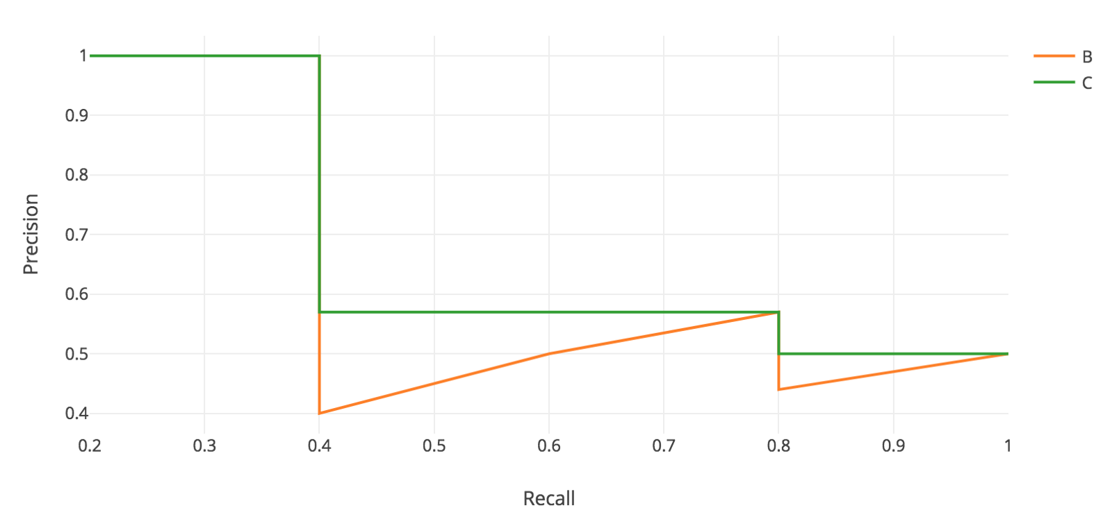The average precision (AP) for this image and class is the area under this smoothed curve.

To compute the mean average precision over the whole dataset, we average the AP for each image and class, giving us one single metric of our network’s performance on classification! This is the metric that is used for common object detection benchmarks such as Pascal VOC and COCO.

Evaluation Metrics for NLP Tasks

• Generative language models
  • Perplexity
  • Cross entropy
• Machine Translation
  • BLEU
  • ROUGE
• Multi-task learning
  • GLUE
• Manual evaluation by humans for fluency, grammar, comparative ranking, etc.

Articles and resources:

• Evaluation Metrics for Language Modeling (article)
• Evaluation Metrics for Language Models (paper)

Evaluations Metrics for GANs

• Inception Score
• Wasserstein distance
• Fréchet Inception Distance
• Traditional metrics such as precision, recall, and F1

Articles and resources:

• An empirical study on evaluation metrics of generative adversarial networks (paper)
• How to measure GAN performance? (blog post)
• Are GANs Created Equal? A Large-Scale Study (paper)
• Pros and Cons of GAN Evaluation Measures (paper)
• How to Evaluate GANs (blog post)