Slides: (slides)
Training a deep neural network involves finding the right values for the weights: we would like to end with a model with good generalization error. Our model should perform well on the full, real-world data distribution, and should neither underfit nor overfit.
In this section, we’ll analyze two methods, initialization and regularization, and show how they help us train models more effectively.
Xavier Initialization
Last week, we discussed backpropagation and gradient descent for deep learning models. All deep learning optimization methods involve an initialization of the weight parameters.
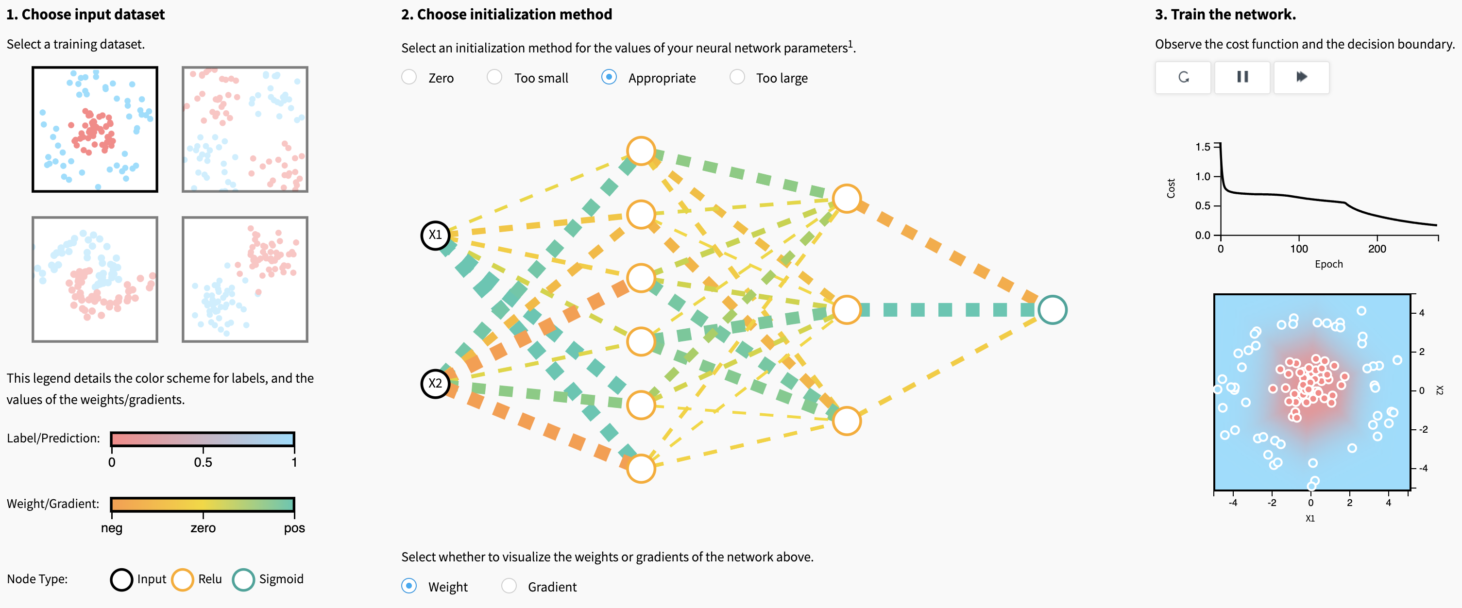
Let’s explore the first visualization in this article to gain some intuition on the effect of different initializations.
What makes a good or bad initialization? How can different magnitudes of initializations lead to exploding and vanishing gradients?
If we initialize weights to all zeros or the same value, what problem arises?
 |
The goal of Xavier Initialization is to initialize the weights such that the variance of the activations are the same across every layer. This constant variance helps prevent the gradient from exploding or vanishing.
To help derive our initialization values, we will make the following simplifying assumptions:
- Weights and inputs are centered at zero
- Weights and inputs are independent and identically distributed
- Biases are initialized as zeros
- We use the tanh() activation function, which is approximately linear with small inputs: \(Var(a^{[l]}) \approx Var(z^{[l]})\)
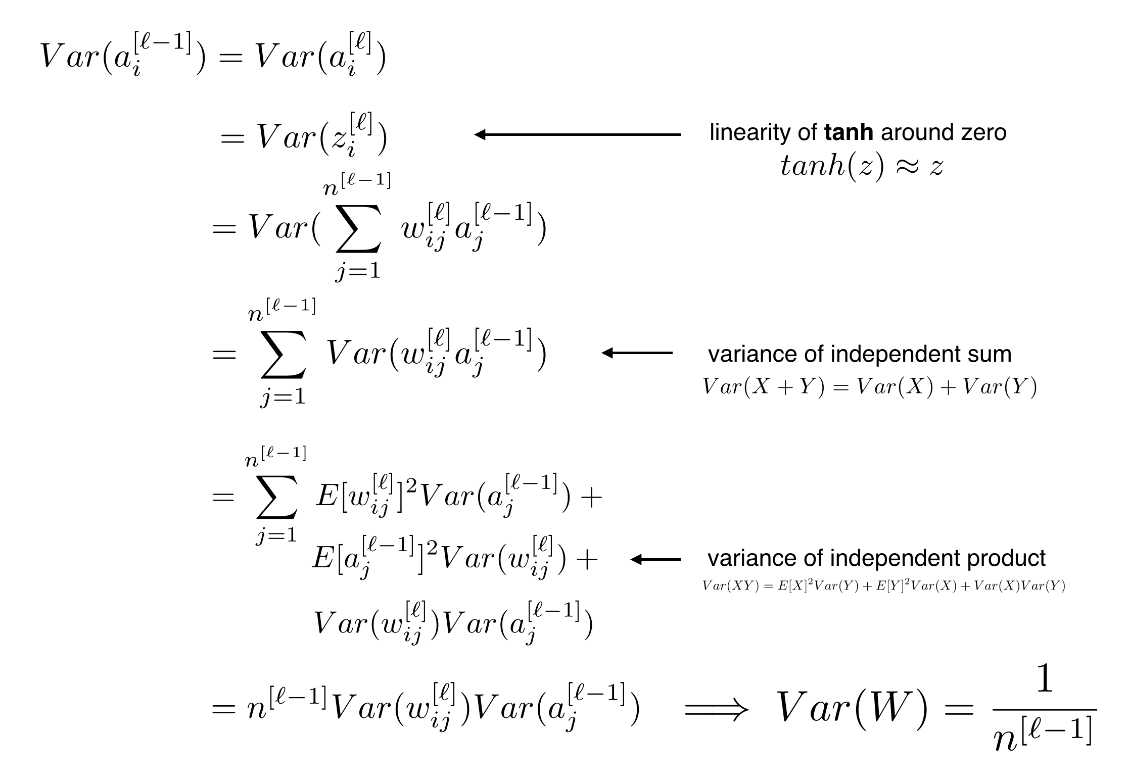
Let’s derive Xavier Initialization now, step by step.
Our full derivation gives us the following initialization rule, which we apply to all weights:
\[W^{[l]}_{i,j} = \mathcal{N}\left(0,\frac{1}{n^{[l-1]}}\right)\] |
Xavier initialization is designed to work well with tanh or sigmoid activation functions. For ReLU activations, look into He initialization, which follows a very similar derivation.
L1 and L2 Regularization
We know that \(L_1\) regularization encourages sparse weights (many zero values), and that \(L_2\) regularization encourages small weight values, but why does this happen?
Let’s consider some cost function \(J(w_1,\dots,w_l)\), a function of weight matrices \(w_1,\dots,w_l\). Let’s define the following two regularized cost functions:
\[\begin{align} J_{L_1}(w_1,\dots,w_l) &= J(w_1,\dots,w_l) + \lambda\sum_{i=1}^l|w_i|\\ J_{L_2}(w_1,\dots,w_l) &= J(w_1,\dots,w_l) + \lambda\sum_{i=1}^l||w_i||^2 \end{align}\]Let’s derive the gradient updates for these cost functions.
The update for \(w_i\) when using \(J_{L_1}\) is:
\[w_i^{k+1} = w_i^{k} - \underbrace{\alpha\lambda sign(w_i)}_{L_1 \text{ penalty}} - \alpha\frac{\partial J}{\partial w_i}\]The update for \(w_i\) when using \(J_{L_2}\) is:
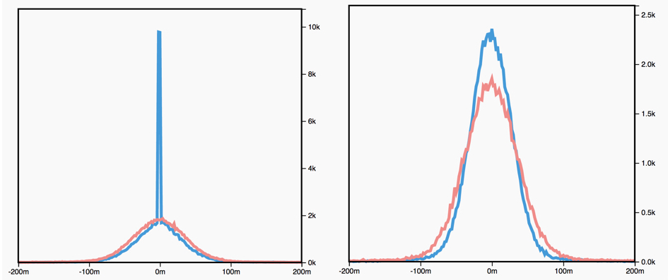
\[w_i^{k+1} = w_i^{k} - \underbrace{2\alpha\lambda w_i}_{L_2 \text{ penalty}}- \alpha\frac{\partial J}{\partial w_i}\]What do you notice that is different between these two update rules, and how does it affect optimization? What effect does the hyperparameter \(\lambda\) have?
 |
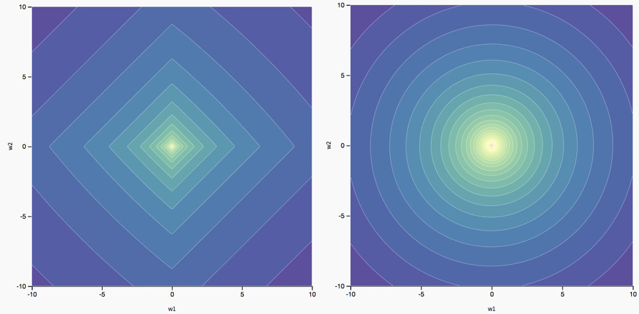
The different effects of \(L_1\) and \(L_2\) regularization on the optimal parameters are an artifact of the different ways in which they change the original loss landscape. In the case of two parameters (\(w_1\) and \(w_2\)), we can visualize this.
 |
For a deeper dive into regularization, take a look at this longer blog post, as well as Chapter 3 of The Elements of Statistical Learning.
 CS230
CS230

