Introduction

When datasets are large and high-dimensional, it is computationally very expensive (sometimes impossible!) to find an analytical solution for the optimal parameters of your network. Instead, we use optimization methods. A vanilla optimization approach would be to sample different combinations of parameters and choose the one with the lowest loss value.

• Is this a good idea?
• Would it be possible to extract another piece of information to direct our search towards the optimal parameters?

The trajectory through a loss landscape for a linear regression model trained with gradient descent. The red dot indicates the value of the loss function corresponding to the initial parameter values. (source)

This is exactly what gradient descent does! Apart from the loss value, gradient descent computes the local gradient of the loss when evaluating potential parameters. This information is used to decide which direction the search should go to find better parameter values. This extra piece of information (the local gradient) can be computed relatively easily using backpropagation. This recursive algorithm breaks up complex derivatives into smaller parts through the chain rule.

To help understand gradient descent, let’s visualize the setup.

Univariate Regression

Let’s consider a linear regression. You have a data set \((x,y)\) with \(m\) examples. In other words, \(x = (x_1,\dots , x_m)\) and \(y = (y_1, \dots, y_m)\) are row vectors of \(m\) scalar examples . The goal is to find the scalar parameters \(w\) and \(b\) such that the line \(y = wx + b\) optimally fits the data. This can be achieved using gradient descent.

Forward Propagation

The first step of gradient descent is to compute the loss. To do this, define your model’s output and loss function. In this regression setting, we use the mean squared error loss.

\[\begin{align} \hat{y} &= wx + b\\\\ \mathcal{L} &= \frac{1}{m}||\hat{y} - y||^2 \end{align}\]

Backward Propagation

The next step is to compute the local gradient of the loss with respect to the parameters (i.e. \(w\) and \(b\)). This means you need to calculate derivatives. Note that values stored during the forward propagation are used in the gradient equations.

\[\begin{align} \frac{\partial\mathcal{L}}{\partial w} &= \frac{2}{m}(\hat{y} - y)x^\intercal\\\\ \frac{\partial\mathcal{L}}{\partial b} &= \frac{2}{m}(\hat{y} - y)\vec{1} \end{align}\]

Multivariate Regression

Now, consider the case where \(X\) is a matrix of shape \((n,m)\) and \(y\) is still a row vector of shape \((1,m)\). Instead of a single scalar value, the weights will be a vector (one element per feature) of shape \((1,n)\). The bias parameter is still a scalar.

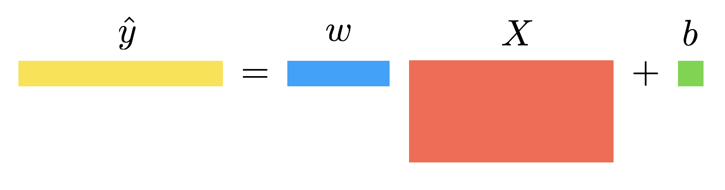Forward Propagation

\[\begin{align} \hat{y} &= wX + b\\\\ \mathcal{L} &= \frac{1}{m}||\hat{y} - y||^2 \end{align}\]

Backward Propagation

\[\begin{align} \frac{\partial\mathcal{L}}{\partial w} &= \frac{2}{m}(\hat{y} - y)X^\intercal\\\\ \frac{\partial\mathcal{L}}{\partial b} &= \frac{2}{m}(\hat{y} - y)\vec{1} \end{align}\]

Two Layer Linear Network

Consider stacking two linear layers together. You can introduce a hidden variable \(Z\) of shape \((k, m)\), which is the output of the first linear layer. The first layer is parameterized by a weight matrix \(W_1\) of shape \((k,n)\) and bias \(b_1\) of shape \((k, 1)\) broadcasted to \((k, m)\). The second layer will be the same as in the multivariate regression case, but its input will be \(Z\) instead of \(X\).

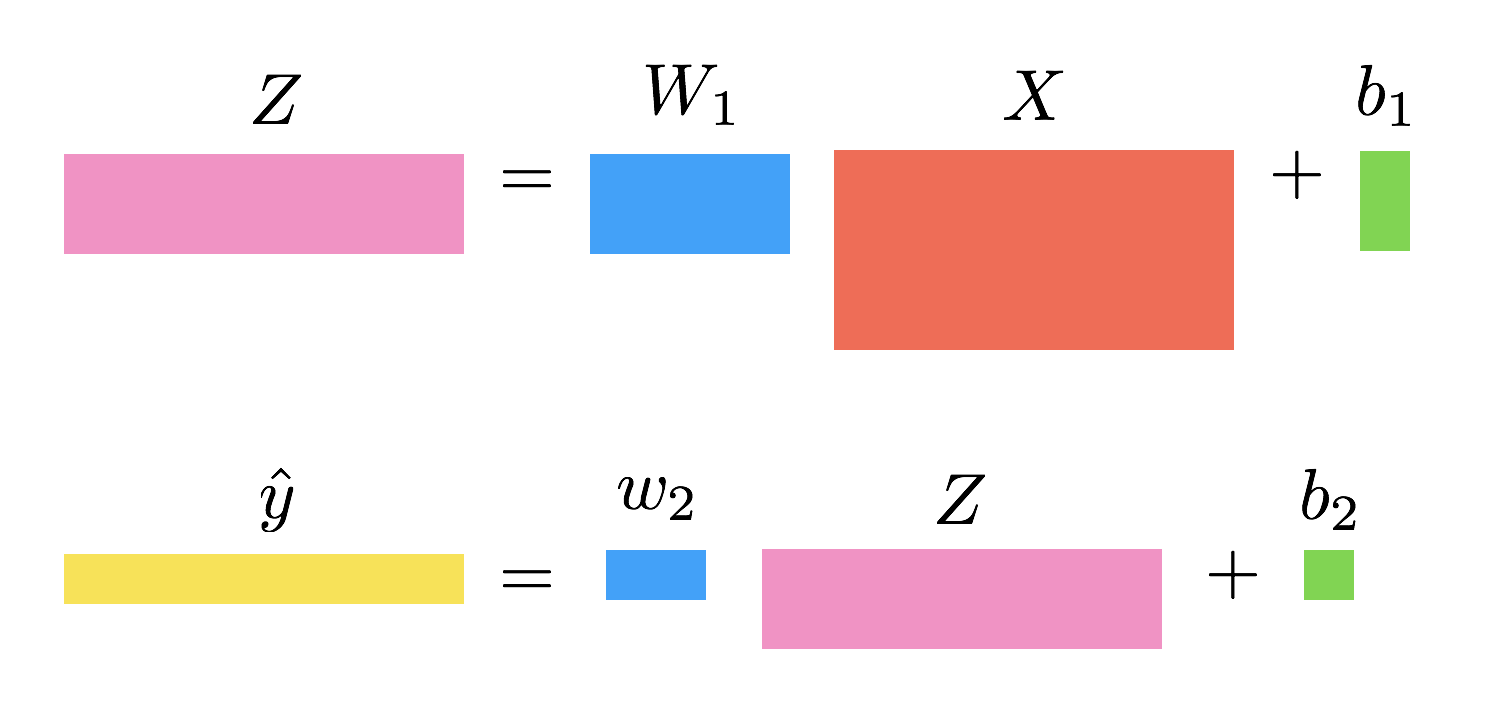Forward Propagation

\[\begin{align} Z &= W_1 X + b_1\\\\ \hat{y} &= w_2Z + b_2\\\\ \mathcal{L} &= \frac{1}{m}||\hat{y} - y||^2 \end{align}\]

Backward Propagation

\[\begin{align} \frac{\partial\mathcal{L}}{\partial W_1} &= w_2^\intercal\frac{2}{m}(\hat{y} - y)X^\intercal\\\\ \frac{\partial\mathcal{L}}{\partial b_1} &= w_2^\intercal\frac{2}{m}(\hat{y} - y)\vec{1}\\\\ \frac{\partial\mathcal{L}}{\partial w_2} &= \frac{2}{m}(\hat{y} - y)Z^\intercal\\\\ \frac{\partial\mathcal{L}}{\partial b_2} &= \frac{2}{m}(\hat{y} - y)\vec{1} \end{align}\]

Two Layer Nonlinear Network

In this example, before sending \(Z\) as the input to the second layer, you will pass it through the sigmoid function. The output is denoted \(A\) and is the input of the second layer.

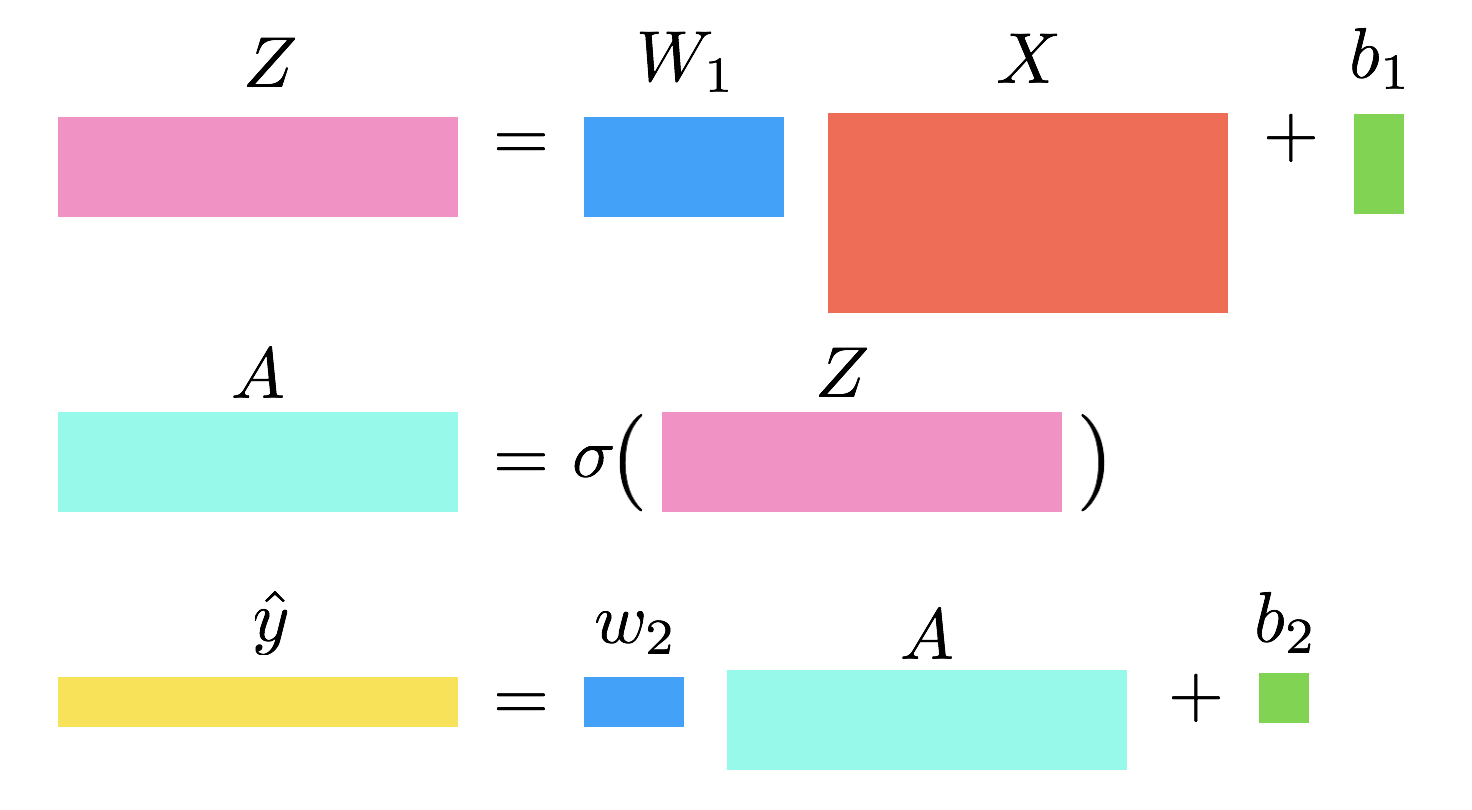Forward Propagation

\[\begin{align} Z &= W_1 X + b_1\\\\ A &= \sigma(Z)\\\\ \hat{y} &= w_2A + b_2\\\\ \mathcal{L} &= \frac{1}{m}||\hat{y} - y||^2 \end{align}\]

Backward Propagation

\[\begin{align} \frac{\partial\mathcal{L}}{\partial W_1} &= \left(\left(w_2^\intercal\frac{2}{m}(\hat{y} - y)\right)\odot A \odot (1 - A)\right)X^\intercal\\\\ \frac{\partial\mathcal{L}}{\partial b_1} &= \left(\left(w_2^\intercal\frac{2}{m}(\hat{y} - y)\right)\odot A \odot (1 - A)\right)\vec{1}\\\\ \frac{\partial\mathcal{L}}{\partial w_2} &= \frac{2}{m}(\hat{y} - y)A^\intercal\\\\ \frac{\partial\mathcal{L}}{\partial b_2} &= \frac{2}{m}(\hat{y} - y)\vec{1} \end{align}\]

Extended Notes

We have compiled an illustrative set of handwritten notes that cover:

• Scalar Operations and their derivatives,
• Detailed visualizations of the backprop calculation for logistic regression and a 2-layer perceptron,
• An overview of common optimization techniques: mini-batch GD, momentum, RMSprop, and Adam.

Exercises

We also put together a sheet of exercises (and their solutions) to help you test your understanding of gradient descent and backpropogation, as well as provide useful practice for the exam.

Even more Resources

• Matrix derivatives “cheat” sheet
• Chapter 7 of CS229 Lecture Notes