For the last section of the quarter, we will be dividing into students and having them provide feedback on each other’s drafts of the final report. Please come prepared!

Hyperparameter Tuning

Lots of hyperparameters are involved in the design of a deep neural network. Finding the best set of hyperparameters is an optimization task in of itself! In most cases, the space of possible hyperparameters is far too large for us to try all of them. Here are some strategies for solving this problem.

Random Search and Grid Search

Consider the following function $f(x,y) = g(x) + h(y)$ over parameters $x,y$ and the maximization problem:

\[\max_{x,y} f(x,y).\]

Assume we only have access to $f(x,y)$ through an oracle (i.e. we can evaluate $f$ at a certain point $(x,y)$, but we do not know the functional form of $f$). How could we find the optimal values of $x$ and $y$?

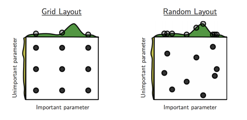
A natural idea would be to choose a range for the values of $x$ and $y$ and sample a grid of points in this range.
We could also evaluate a numerical gradient in the hyperparameter space. The challenge with this method is that unlike an iteration of model training, each evaluation of hyperparameters is very costly and long, making it infeasible to try many combinations of hyperparameters.

Now assume we know that

\[f(x,y) = g(x) + h(y) \approx g(x).\]

Would grid search still be a good strategy?

The function $f$ mostly depends on $x$. Thus, a grid search strategy will waste a lot of iterations testing different values of $y$. If we have a finite number of evaluations of $(x,y)$, a better strategy would be randomly sampling $x$ and $y$ in a certain range, that way each sample tests a different value of each hyperparameter.

An illustration of how random search can improve on grid search of hyperparameters. 'This failure of grid search is the rule rather than the exception in high dimensional hyperparameter optimization.' (Bergstra & Bengio, 2011). (source)

What are weaknesses and assumptions of random search?

Random search assumes that the hyperparameters are uncorrelated. Ideally, we would sample hyperparameters from a joint distribution that takes into account this understanding. Additionally, it doesn’t use the results of previous iterations to inform how we choose parameter values for future iterations. This is the motivation behind Bayesian optimization.

Bayesian Optimization

Bayesian inference is a form of statistical inference that uses Bayes’ Theorem to incorporate prior knowledge when performing estimation. Bayes’ Theorem is a simple, yet extremely powerful, formula relating conditional and joint distributions of random variables. Let $X$ be the random variable representing the quality of our model and $\theta$ the random variable representing our hyperparameters. Then Bayes’ Rule relates the distributions $p(\theta \mid X)$ (posterior), $p(X\mid\theta)$ (likelihood), $p(\theta)$ (prior) and $p(X)$ (marginal) as:

\[p(\theta\mid M) = \frac{p(M \mid \theta)p(\theta)}{p(M)}\]

How could we use Bayes’ Rule to improve random search?

By using a prior on our hyperparameters, we can incorporate prior knowledge into our optimizer. By sampling from the posterior distribution instead of a uniform distribution, we can incorporate the results of our previous samples to improve our search process.

Let’s reconsider the optimization problem of finding the maximum of $f(x,y)$. A Bayesian optimization strategy would:

Initialize a prior on the parameters $x$ and $y$.
Sample an point $(x,y)$ to evaluate $f$ with.
Use the result of $f(x,y)$ to update the posterior on $x,y$.
Repeat 2 and 3.

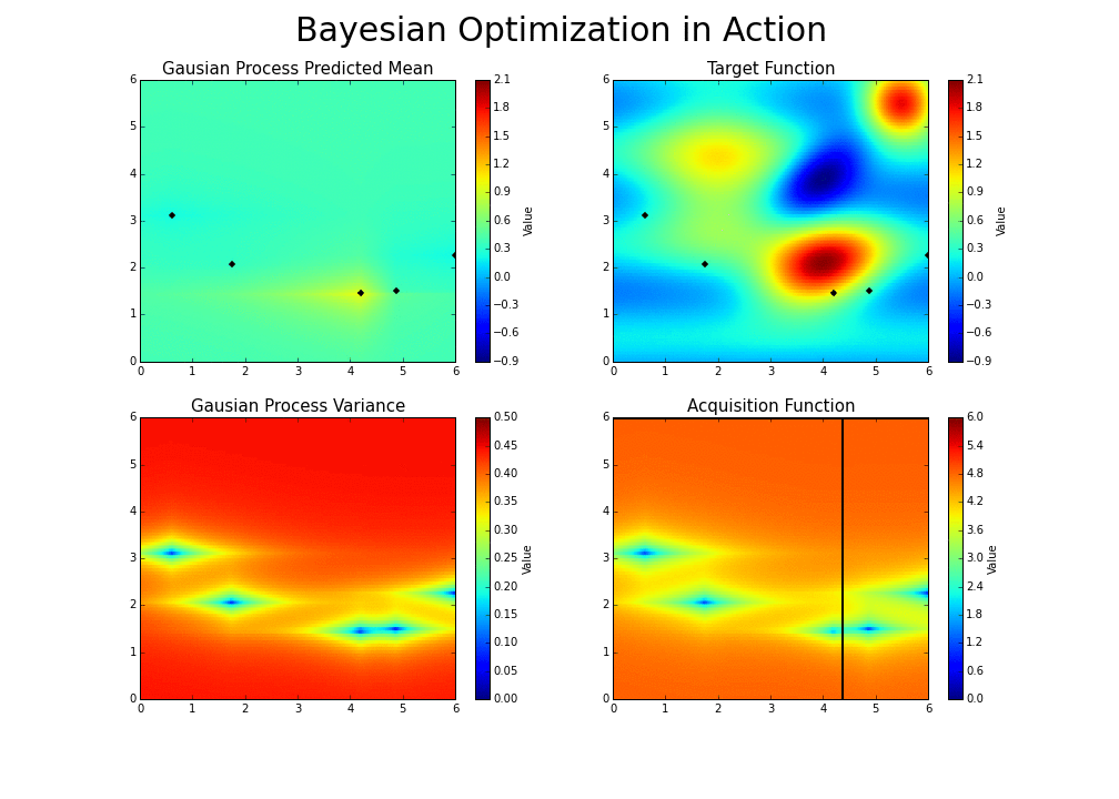
The goal is to guess the function, even if we cannot know its true form. By adding a new data point at each iteration, the algorithm can guess the function more accurately, and more intelligently choose the next point to evaluate to improve its guess. A Gaussian process is used to infer the function from samples of its inputs and outputs. It also provides a distribution over the possible functions given the observed data.

Let’s consider an example: say we want to find the minimum of some function whose expression is unknown. The function has one input and one output, and we’ve taken four different samples (the blue points).

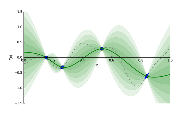A Gaussian process distribution, given four sampled data points in blue. (source)

The Gaussian process provides a distribution of continuous functions that fit these points, which is represented in green. The darker the shade, the more likely the true function is within that region. The green line is the mean guess of the “true” function, and each band of green is a half standard deviation of the Gaussian process distribution.

Now, given this useful guess, what point should we evaluate next? We have two possible options:

Exploitation: Evaluate a point that, based on our current model of likely functions, will yield a low output value. For instance, 1.0 could be an option in the above graph.
Exploration: Get a datapoint on an area we’re most unsure about. In the graph above, we could focus on the zone between .65 and .75, rather than between .15 and .25, since we have a pretty good idea as to what’s going on in the latter zone. That way, we will will be able to reduce the variance of future guesses.

Balancing these two is the exploration-exploitation trade-off. We choose between the two strategies using an acquisition function.

With each iteration 'the algorithm balances its needs of exploration and exploitation' (Nogueira). (source)

If you’re interested in learning more or trying out the optimizer, here is a good Python code base for using Bayesian Optimization with Gaussian processes.

TensorBoard

TensorBoard is a great way to track and visualize neural network performance over time as it trains!

TensorBoard. (source)

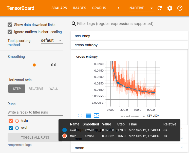TensorBoard was built for TensorFlow, but can also be used with PyTorch using the TensorBoardX library.

Let’s walk through the AWS TensorBoard code and see it in action on an AWS instance. Instructions here. Make sure to perform steps 5 and 6 (opening a port in your AWS security settings, and setting up an SSH tunnel to your machine).

Running TensorBoard Locally

We’ve also created a few Tensorflow 2/Keras examples that you can run on your local machine. These examples demonstrate how to show how to display loss curves, images, and figures like confusion matrices for the MNIST classification task on your local machine.

Setup

You’ll need a couple of python packages to get started with these examples. Run these commands to create a virtual environment for this tutorial and start a TensorBoard server:

virtualenv -p python3 .venv
source .venv/bin/activate
pip install numpy matplotlib tensorflow tensorboard scikit-learn
tensorboard --logdir logs &

Running tensorboard --logdir logs & will create a directory called logs where TensorBoard will store the metrics from your training runs and start a TensorBoard server as a background process. Open the TensorBoard dashboard by going to localhost:6006 in your browser (or whichever port number your server is running on).

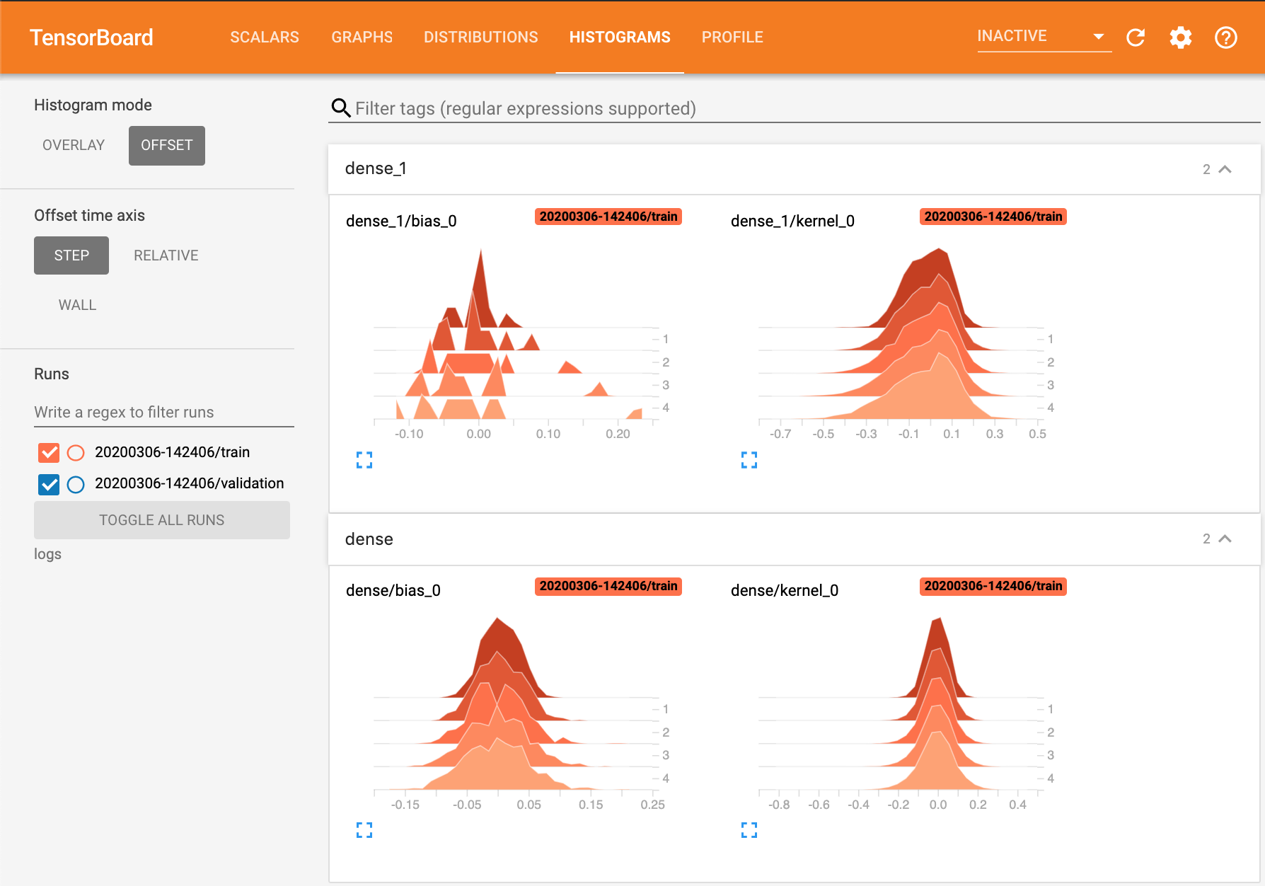
Plotting losses, accuracies, and weight distributions

For this first example we’ll plot train and val loss and accuracy curves in addition to histograms of the weights of our network as it trains. To do this, we import the TensorBoard callback, configure where it will store the training logs (we name this directory as a formatted string representing the current time), and pass this callback to model.fit():

import datetime
import tensorflow as tf
from tensorflow.keras.datasets import mnist
from tensorflow.keras.models import Sequential
from tensorflow.keras.layers import Flatten, Dense, Dropout
from tensorflow.keras.callbacks import TensorBoard

(x_train, y_train), (x_test, y_test) = mnist.load_data()
x_train, x_test = x_train / 255.0, x_test / 255.0

model = Sequential([
    Flatten(input_shape=(28, 28)),
    Dense(512, activation='relu'),
    Dropout(0.2),
    Dense(10, activation='softmax')
])
model.compile(optimizer='adam',
              loss='sparse_categorical_crossentropy',
              metrics=['accuracy'])

time = datetime.datetime.now().strftime("%Y%m%d-%H%M%S")
log_dir = f"logs/{time}"
tensorboard = TensorBoard(log_dir=log_dir, histogram_freq=1) # added

model.fit(
    x=x_train,
    y=y_train,
    epochs=5,
    validation_data=(x_test, y_test),
    callbacks=[tensorboard]
    )

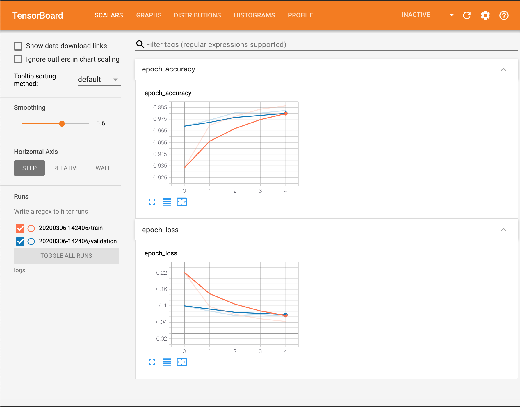We can see plots of the train and val losses and accuracies by navigating to the 'Scalars' tab of the TensorBoard dashboard at 'localhost:6000' in a browser. (source)

By setting histogram_freq=1 in the TensorBoard callback constructor, we can track the distributions of the weights in each layer at each epoch.

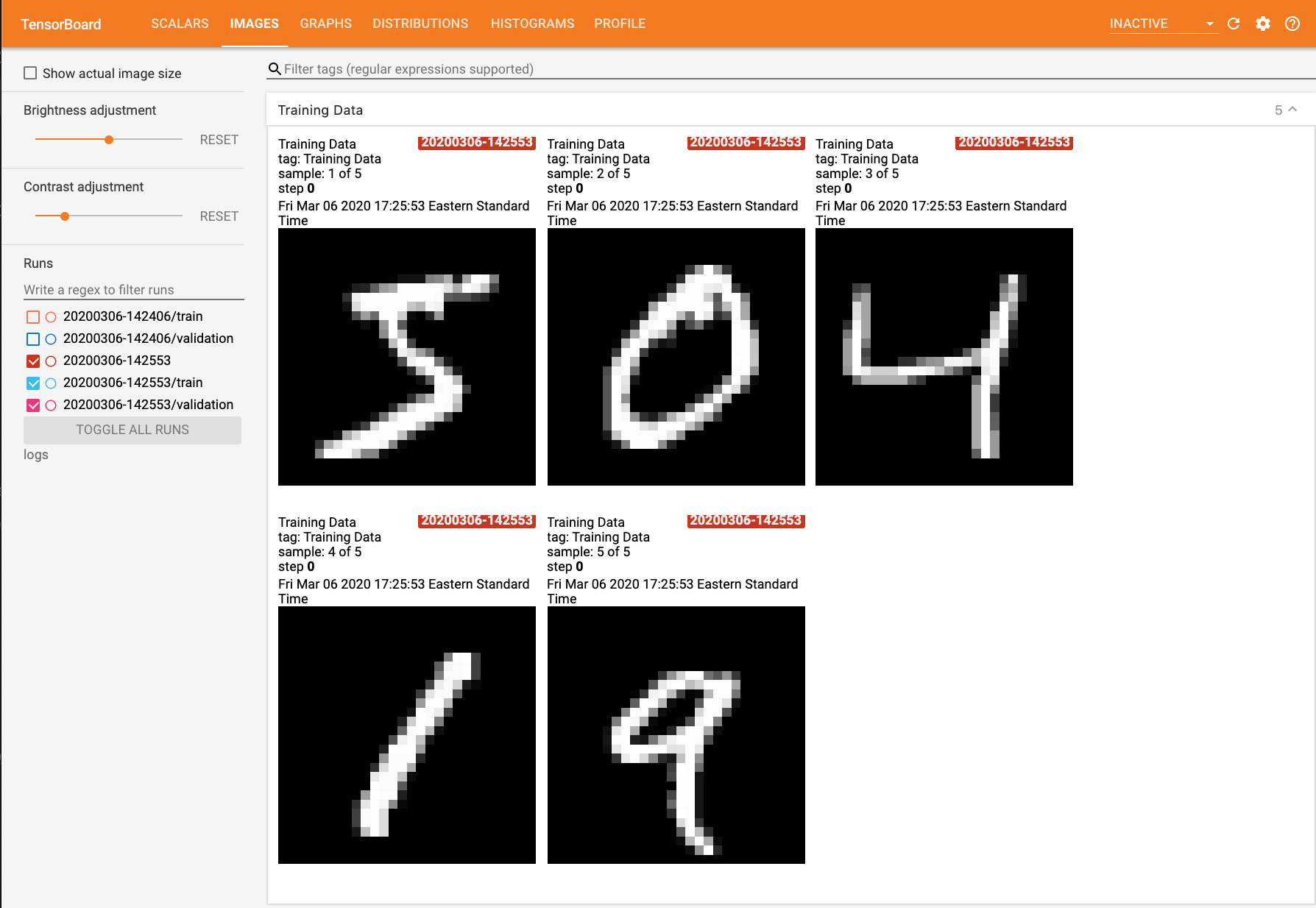
The 'Histograms' tab shows histograms of the weights in each layer at each epoch. (source)

Logging Images

This next example shows how to use tf.summary to log image data for visualization. Here we simply log the first five examples in the training set so that we can inspect them in the ‘Images’ tab of the TensorBoard dashboard.

import datetime
import tensorflow as tf
from tensorflow.keras.datasets import mnist
from tensorflow.keras.models import Sequential
from tensorflow.keras.layers import Flatten, Dense, Dropout
from tensorflow.keras.callbacks import TensorBoard

import matplotlib.pyplot as plt # added
import numpy as np # added
import sklearn.metrics # added

(x_train, y_train), (x_test, y_test) = mnist.load_data()
x_train, x_test = x_train / 255.0, x_test / 255.0

time = datetime.datetime.now().strftime("%Y%m%d-%H%M%S")
log_dir = f"logs/{time}"
tensorboard = TensorBoard(log_dir=log_dir, histogram_freq=1)

# Visualize image, added
images = np.reshape(x_train[0:5], (-1, 28, 28, 1)) # batch_size first
file_writer = tf.summary.create_file_writer(log_dir)
with file_writer.as_default():
	tf.summary.image("Training Data", images, max_outputs=5, step=0)

model = Sequential([
    Flatten(input_shape=(28, 28)),
    Dense(512, activation='relu'),
    Dropout(0.2),
    Dense(10, activation='softmax')
])
model.compile(optimizer='adam',
              loss='sparse_categorical_crossentropy',
              metrics=['accuracy'])

model.fit(
    x=x_train, 
    y=y_train, 
    epochs=5, 
    validation_data=(x_test, y_test), 
    callbacks=[tensorboard]
)

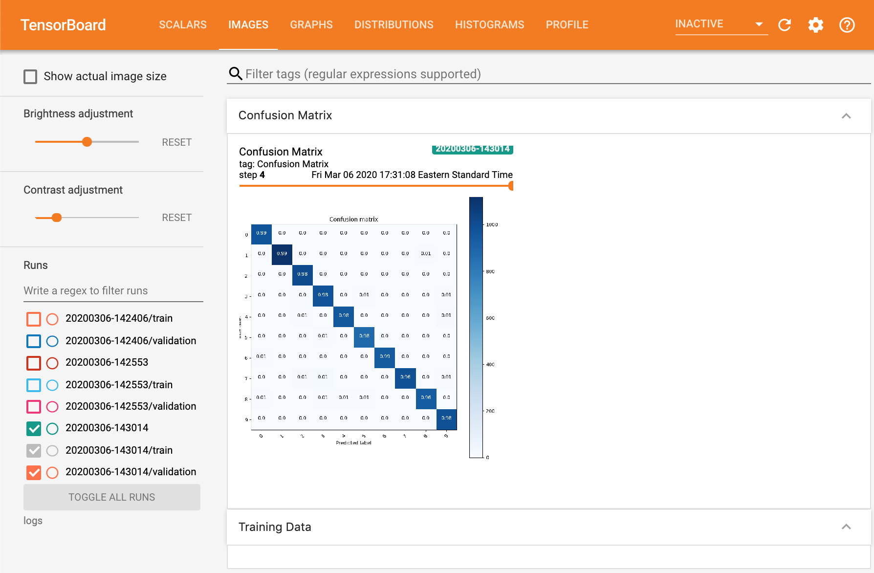
Custom Logging Callbacks

The previous example showed how to log images from the training set at the beginning of training, but it would be more helpful to be able to log images and figures continusouly over the course of training. For example, if we were training a GAN, monitoring the loss curves of the generator and discriminator over time wouldn’t give much insight into the performance of the model, and it would be much more illuminating to be able to view samples generated over time to see if sample quality is improving. Likewise, for a classification task like MNIST digit classification, being able to see the evolution of confusion matrices or ROC curves over time can give a better sense of model performance than a single number like accuracy. Here we show how to plot confusion matrices at the end of each epoch.

We can define custom logging behavior that executes at fixed intervals during training using a LambdaCallback. In the code below, we define a function log_confusion_matrix that generates the model’s predictions on the val set and creates a confusion matrix image using the sklearn.metrics.confusion_matrix() function, and create a callback that plots the confusion matrix at the end of every epoch with cm_callback = LambdaCallback(on_epoch_end=log_confusion_matrix).

import datetime
import tensorflow as tf
from tensorflow.keras.datasets import mnist
from tensorflow.keras.models import Sequential
from tensorflow.keras.layers import Flatten, Dense, Dropout
from tensorflow.keras.callbacks import TensorBoard, LambdaCallback # added

import io # added
import itertools # added
import matplotlib.pyplot as plt
import numpy as np
import sklearn.metrics

# Added
def plot_to_image(fig):
	buf = io.BytesIO()
	plt.savefig(buf, format='png')
	plt.close(fig)
	buf.seek(0)
	img = tf.image.decode_png(buf.getvalue(), channels=4)
	img = tf.expand_dims(img, 0)
	return img

# Added
def plot_confusion_matrix(cm, class_names):
	figure = plt.figure(figsize=(8, 8))
	plt.imshow(cm, interpolation='nearest', cmap=plt.cm.Blues)
	plt.title("Confusion matrix")
	plt.colorbar()
	tick_marks = np.arange(len(class_names))
	plt.xticks(tick_marks, class_names, rotation=45)
	plt.yticks(tick_marks, class_names)

	cm = np.around(cm.astype('float') / cm.sum(axis=1)[:, np.newaxis], decimals=2)

	threshold = cm.max() / 2.
	for i, j in itertools.product(range(cm.shape[0]), range(cm.shape[1])):
		color = "white" if cm[i, j] > threshold else "black"
		plt.text(j, i, cm[i, j], horizontalalignment="center", color=color)

	plt.tight_layout()
	plt.ylabel('True label')
	plt.xlabel('Predicted label')
	return figure

(x_train, y_train), (x_test, y_test) = mnist.load_data()
x_train, x_test = x_train / 255.0, x_test / 255.0

time = datetime.datetime.now().strftime("%Y%m%d-%H%M%S")
log_dir = f"logs/{time}"
tensorboard = TensorBoard(log_dir=log_dir, histogram_freq=1)

# Added
file_writer = tf.summary.create_file_writer(log_dir)
def log_confusion_matrix(epoch, logs):
	test_pred_raw = model.predict(x_test)
	test_pred = np.argmax(test_pred_raw, axis=1)

	cm = sklearn.metrics.confusion_matrix(y_test, test_pred)
	figure = plot_confusion_matrix(cm, class_names=list(range(10)))
	cm_image = plot_to_image(figure)
	with file_writer.as_default():
		tf.summary.image("Confusion Matrix", cm_image, step=epoch)
cm_callback = LambdaCallback(on_epoch_end=log_confusion_matrix)

model = Sequential([
    Flatten(input_shape=(28, 28)),
    Dense(512, activation='relu'),
    Dropout(0.2),
    Dense(10, activation='softmax')
])
model.compile(optimizer='adam',
              loss='sparse_categorical_crossentropy',
              metrics=['accuracy'])

model.fit(
    x=x_train, 
    y=y_train, 
    epochs=5, 
    validation_data=(x_test, y_test), 
    callbacks=[tensorboard, cm_callback] # added
)

LambdaCallbacks allow us to view the history of confusion matrices summarizing our model's performance on the val set over time (source)

Section 9 (Week 9)

Instructors

Time and Location