Create and train a Model

This post is part of a series of post explaining how to structure a deep learning project in TensorFlow. We will explain here how to easily define a deep learning model in TensorFlow using tf.layers, and how to train it. The entire code examples can be found in our github repository.

This tutorial is among a series explaining how to structure a deep learning project:

installation, get started with the code for the projects
(TensorFlow only): explain the global structure of the code
(TensorFlow only): how to feed data into the model using tf.data
this post: how to create the model and train it

Goals of this tutorial

learn more about TensorFlow
learn how to easily build models using tf.layers
…

Defining the model

Great, now we have this input dictionnary containing the Tensor corresponding to the data, let’s explain how we build the model.

Introduction to tf.layers

This high-level Tensorflow API lets you build and prototype models in a few lines. You can have a look at the official tutorial for computer vision, or at the list of available layers. The idea is quite simple so we’ll just give an example.

Let’s get an input Tensor with a similar mechanism than the one explained in the previous part. Remember that None corresponds to the batch dimension.

#shape = [None, 64, 64, 3]
images = inputs["images"]

Now, let’s apply a convolution, a relu activation and a max-pooling. This is as simple as

out = images
out = tf.layers.conv2d(out, 16, 3, padding='same')
out = tf.nn.relu(out)
out = tf.layers.max_pooling2d(out, 2, 2)

Finally, use this final tensor to predict the labels of the image (6 classes). We first need to reshape the output of the max-pooling to a vector

#First, reshape the output into [batch_size, flat_size]
out = tf.reshape(out, [-1, 32 * 32 * 16])
#Now, logits is [batch_size, 6]
logits = tf.layers.dense(out, 6)

Note the use of -1: Tensorflow will compute the corresponding dimension so that the total size is preserved.

The logits will be unnormalized scores for each example.

In the code examples, the transformation from inputs to logits is done in the build_model function.

Training ops

At this point, we have defined the logits of the model. We need to define our predictions, our loss, etc. You can have a look at the model_fn in model/model_fn.py.

#Get the labels from the input data pipeline
labels = inputs['labels']
labels = tf.cast(labels, tf.int64)

#Define the prediction as the argmax of the scores
predictions = tf.argmax(logits, 1)

#Define the loss
loss = tf.losses.sparse_softmax_cross_entropy(labels=labels, logits=logits)

The 1 in tf.argmax tells Tensorflow to take the argmax on the axis = 1 (remember that axis = 0 is the batch dimension)

Now, let’s use Tensorflow built-in functions to create nodes and operators that will train our model at each iteration !

#Create an optimizer that will take care of the Gradient Descent
optimizer = tf.train.AdamOptimizer(0.01)

#Create the training operation
train_op = optimizer.minimize(loss)

All these nodes are created by model_fn that returns a dictionnary model_spec containing all the necessary nodes and operators of the graph. This dictionnary will later be used for actually running the training operations etc.

And that’s all ! Our model is ready to be trained. Remember that all the objects we defined so far are nodes or operators that are part of the Tensorflow graph. To evaluate them, we actually need to execute them in a session. Simply run

with tf.Session() as sess:
    for i in range(num_batches):
        _, loss_val = sess.run([train_op, loss])

Notice how we don’t need to feed data to the session as the tf.data nodes automatically iterate over the dataset ! At every iteration of the loop, it will move to the next batch (remember the tf.data part), compute the loss, and execute the train_op that will perform one update of the weights !

For more details, have a look at the model/training.py file that defines the train_and_evaluate function.

Putting input_fn and model_fn together

To summarize the different steps, we just give a high-level overview of what needs to be done in train.py

#1. Create the iterators over the Training and Evaluation datasets
train_inputs = input_fn(True, train_filenames, train_labels, params)
eval_inputs = input_fn(False, eval_filenames, eval_labels, params)

#2. Define the model
logging.info("Creating the model...")
train_model_spec = model_fn('train', train_inputs, params)
eval_model_spec = model_fn('eval', eval_inputs, params, reuse=True)

#3. Train the model (where a session will actually run the different ops)
logging.info("Starting training for {} epoch(s)".format(params.num_epochs))
train_and_evaluate(train_model_spec, eval_model_spec, args.model_dir, params, args.restore_from)

The train_and_evaluate function performs a given number of epochs (= full pass on the train_inputs). At the end of each epoch, it evaluates the performance on the development set (dev or train-dev in the course material).

Remember the discussion about different graphs for Training and Evaluation. Here, notice how the eval_model_spec is given the reuse=True argument. It will make sure that the nodes of the Evaluation graph which must share weights with the Training graph do share their weights.

Evalution and tf.metrics

Tensorflow doc

So far, we’ve explained how we input data to the graph, how we define the different nodes and training ops, but we don’t know (yet) how to compute some metrics on our dataset. There are basically 2 possibilities

[run evaluation outside the Tensorflow graph] Evaluate the prediction over the dataset by running sess.run(prediction) and use it to evaluate your model (without Tensorflow, with pure python code). This option can also be used if you need to write a file with all the predicitons and use a script (distributed by a conference for instance) to evaluate the performance of your model.
[use Tensorflow] As the above method can be quite complicated for simple metrics, Tensorflow luckily has some built-in tools to run evaluation. Again, we are going to create nodes and operations in the Graph. The concept is simple: we will use the tf.metrics API to build those, the idea being that we need to update the metric on each batch. At the end of the epoch, we can just query the updated metric !

We’ll cover method 2 as this is the one we implemented in the code examples (but you can definitely go with option 1 by modifying model/evaluation.py). As most of the nodes of the graph, we define these metrics nodes and ops in model/model_fn.py.

#Define the different metrics
with tf.variable_scope("metrics"):
    metrics = {'accuracy': tf.metrics.accuracy(labels=labels, predictions=predictions,
              'loss': tf.metrics.mean(loss)}

#Group the update ops for the tf.metrics, so that we can run only one op to update them all
update_metrics_op = tf.group(*[op for _, op in metrics.values()])

#Get the op to reset the local variables used in tf.metrics, for when we restart an epoch
metric_variables = tf.get_collection(tf.GraphKeys.LOCAL_VARIABLES, scope="metrics")
metrics_init_op = tf.variables_initializer(metric_variables)

Notice that we define the metrics, a grouped update op and an initializer. The use of the * in tf.group is a pythonic way to tell that the argument given to the function corresponds to an optional positional argument.

Notice also how we define the metrics in a special variable_scope so that we can query the variables by name when we create the initializer ! When you create nodes, the variables are added to some pre-defined collections of variables (TRAINABLE_VARIABLES, etc.). The variables we need to reset for tf.metrics are in the tf.GraphKeys.LOCAL_VARIABLES collection. Thus, to query the variables, we get the collection of variables in the right scope !

Now, to evaluate the metrics on a dataset, we’ll just need to run them in a session as we loop over our dataset

with tf.Session() as sess:
    #Run the initializer to reset the metrics to zero
    sess.run(metrics_init_op)

    #Update the metrics over the dataset
    for _ in range(num_steps):
        sess.run(update_metrics_op)

    #Get the values of the metrics
    metrics_values = {k: v[0] for k, v in metrics.items()}
    metrics_val = sess.run(metrics_values)

And that’s all ! If you want to compute new metrics for which you can find a Tensorflow implementation, you can define it in the model_fn.py (add it to the metrics dictionnary). It will automatically be updated during the training and will be displayed at the end of each epoch.

Tensorflow Tips and Tricks

Be careful with initialization

So far, we mentionned 3 different initializer operators.

#1. For all the variables (the weights etc.)
tf.global_variables_initializer()

#2. For the dataset, so that we can chose to move the iterator back at the beginning
iterator = dataset.make_initializable_iterator()
next_element = iterator.get_next()
iterator_init_op = iterator.initializer

#3. For the metrics variables, so that we can reset them to 0 at the beginning of each epoch
metrics_init_op = tf.variables_initializer(metric_variables)

During train_and_evaluate we perform the following schedule, all in one session

Loop over the training set, updating the weights and computing the metrics
Loop over the evaluation set, computing the metrics
Go back to step 1.

We thus need to run

tf.global_variable_initializer() at the very beginning (before the first occurence of step 1)
iterator_init_op at the beginning of every loop (step 1 and step 2)
metrics_init_op at the beginning of every loop (step 1 and step 2), to reset the metrics to zero (we don’t want to compute the metrics averaged over the different epochs or different datasets !)

You can indeed check that this is what we do in model/evaluation.py or model/training.py when we actually run the graph !

Saving

Official guide

Training a model and evaluating is fine, but what about re-using the weights? Also, maybe at some point of the training, our performance started to get worse on the validation set and we want to use the best weights we got during training.

Saving models is easy in Tensorflow. Look at the outline below

#We need to create an instance of saver
saver = tf.train.Saver()

for epoch in range(10):
    for batch in range(10):
        _ = sess.run(train_op)

    #Save weights
    save_path = os.path.join(model_dir, 'last_weights', 'after-epoch')
    saver.save(sess, last_save_path, global_step=epoch + 1)

There is not much to say, except that the saver.save() method takes a session as input. In our implementation, we use 2 savers. A last_saver = tf.train.Saver() that will keep the weights at the end of the last 5 epochs and a best_saver = tf.train.Saver(max_to_keep=1) that only keeps one checkpoint corresponding to the weights that achieved the best performance on the validation set !

Later on, to restore the weights of your model, you need to reload the weights thanks to a saver instance, as in

with tf.Session() as sess:
    #Get the latest checkpoint in the directory
    restore_from = tf.train.latest_checkpoint("model/last_weights")
    #Reload the weights into the variables of the graph
    saver.restore(sess, restore_from)

You can look at the files model/training.py and model/evaluation.py for more details.

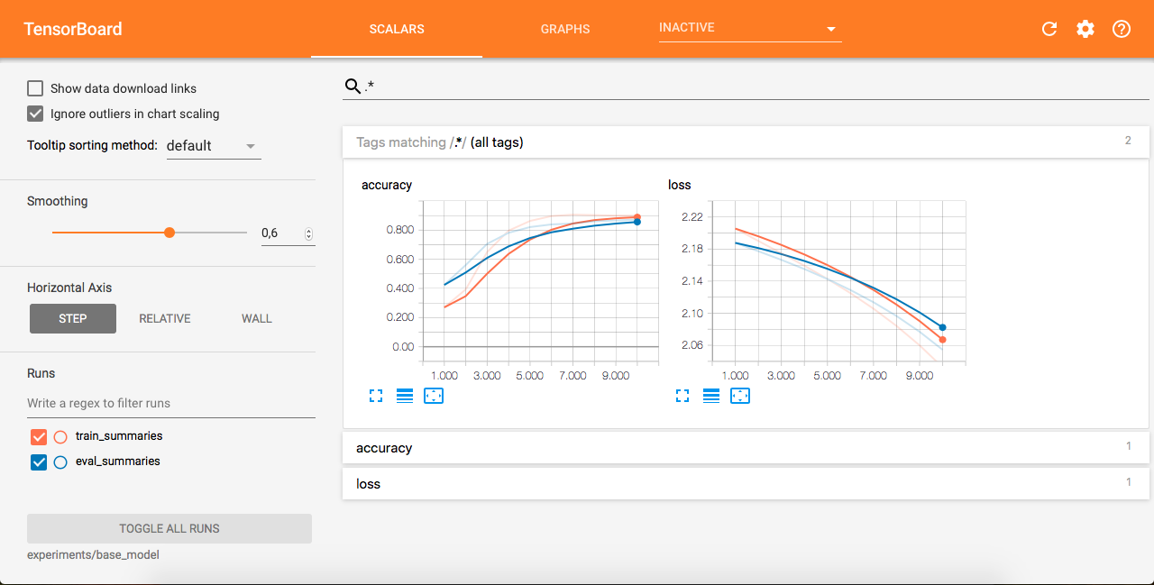
Tensorboard and summaries

Official guide

Tensorflow comes with an excellent visualization tool called Tensorboard that enables you to plot different scalars (and much more) in real-time, as you train your model.

The mechanism of Tensorboard is the following

define some summaries (nodes of the graph) that will tell Tensorflow which values we want to plot
evaluate these nodes in the session
write the output to a file thanks to a tf.summary.FileWriter

Then, you only need to launch tensorboard in your web-browser by opening a terminal and writing for instance

tensorboard --logdir="expirements/base_model"

Then, navigate to http://127.0.0.1:6006/ and you’ll see the different plots.

In the code examples, we add the summaries in model/model_fn.py.

#Compute different scalars to plot
loss = tf.reduce_mean(losses)
accuracy = tf.reduce_mean(tf.cast(tf.equal(labels, predictions), tf.float32))

#Summaries for training
tf.summary.scalar('loss', loss)
tf.summary.scalar('accuracy', accuracy)

Note that we don’t use the metrics that we defined earlier. The reason being that the tf.metrics returns the running average, but Tensorboard already takes care of the smoothing, so we don’t want to add any additional smoothing. It’s actually rather the opposite: we are interested in real-time progress

Once these nodes are added to the model_spec dictionnary, we need to evaluate them in a session. In our implementation, this is done every params.save_summary_steps as you’ll notice in the model/training.py file.

if i % params.save_summary_steps == 0:
    #Perform a mini-batch update
    _, _, loss_val, summ, global_step_val = sess.run([train_op, update_metrics, loss, summary_op, global_step])
    #Write summaries for tensorboard
    writer.add_summary(summ, global_step_val)

else:
    _, _, loss_val = sess.run([train_op, update_metrics, loss])

You’ll notice that we have 2 different writers

train_writer = tf.summary.FileWriter(os.path.join(model_dir, 'train_summaries'), sess.graph)
eval_writer = tf.summary.FileWriter(os.path.join(model_dir, 'eval_summaries'), sess.graph)

They’ll write summaries for both the training and the evaluation, letting you plot both plots on the same graph !

A note about the global_step

Official doc

In order to keep track of how far we are in the training, we use one of Tensorflow’s training utilities, the global_step. Once initialized, we give it to the optimizer.minimize() as explained below. Thus, each time we will run sess.run(train_op), it will increment the global_step by 1. This is very useful for summaries (notice how in the Tensorboard part we give the global step to the writer).

global_step = tf.train.get_or_create_global_step()
train_op = optimizer.minimize(loss, global_step=global_step)

Create and train a Model

Instructors

Time and Location

Goals of this tutorial

Defining the model

Tensorflow Tips and Tricks